Water Viscosity vs Temperature – Table & Formula

Understanding the Viscosity of Water – Core Insights for Chemical and Process Engineers

Water is the most versatile and essential fluid in chemical engineering. It operates as the fundamental solvent, coolant, cleaning medium, and transport mechanism in almost every factory and process plant. The behavior of water—especially its viscosity—directly affects equipment sizing, process safety, energy efficiency, and operational reliability.

Despite its importance, viscosity is frequently underestimated or applied using oversimplified constants, resulting in incorrect pump sizing, excessive pressure drops, suboptimal mixing, and even system failures.

This article provides process engineers, designers, and operators a complete reference for understanding, calculating, and applying water viscosity—including temperature and pressure effects, measurement methods, typical process impacts, and hands-on design examples. By referencing up-to-date data and advanced research, you’ll resolve design risks and optimize equipment for all conditions.

---

What is Viscosity? Key Physical Concepts

Viscosity expresses a fluid’s “thickness” or resistance to deformation. In engineering, two viscosity types are referenced:

1. Dynamic (Absolute) Viscosity ($\mu$)

Measures a fluid’s resistance to shear (internal friction).

Units: Pa·s (Pascal-seconds) or more commonly mPa·s (millipascal-seconds), where
$1~\text{mPa}\cdot\text{s}= 1~\text{cP}$
(centipoise).

2. Kinematic Viscosity ($\nu$)

Ratio of absolute viscosity to density, used for flow calculations such as Reynolds number:

$$\nu = \frac{\mu}{\rho}$$

where:

• $\mu$ = dynamic viscosity [Pa·s]
• $\rho$ = density [kg/m³]
• $\nu$ = kinematic viscosity [m²/s] or [mm²/s] (cSt)

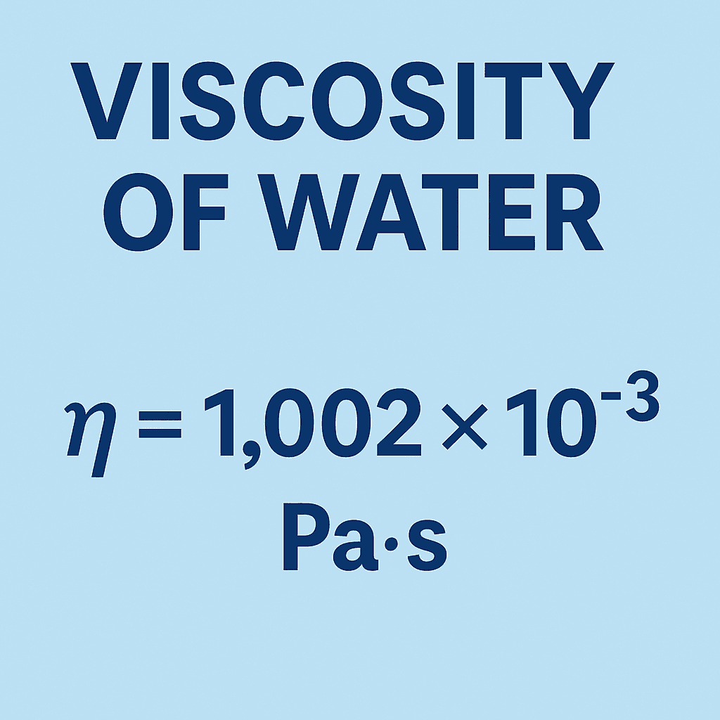
Example properties at 20 °C, 1 atm:

Property	Value	Units
Dynamic Viscosity ($\mu$)	1.002	mPa·s (cP)
Density ($\rho$)	998.2	kg/m³
Kinematic Viscosity ($\nu$)	1.004	mm²/s (cSt)

Water is a Newtonian fluid: its viscosity is independent of shear rate under normal conditions. Thus, viscosity can be treated as a function of temperature and pressure only.

---

Insights on Viscosity Units

While SI and cgs units are both encountered, process engineers should remember:

$1~\text{mPa}\cdot\text{s} = 1000~\text{mPa}\cdot\text{s} = 1000~\text{cP}$
$1~\text{mm}^2/\text{s} = 1~\text{cSt}$

Always clarify units used in design documents—misconversions between cP and mPa·s can cause major calculation errors.

---

How Temperature Dominates Water Viscosity

Water’s viscosity decreases rapidly as temperature rises. Increased molecular kinetic energy weakens hydrogen bonding, reducing internal friction:

$\text{Viscosity} \propto e^{-\text{Temperature}}$

Temperature (°C)	$\mu$ (mPa·s)
0	1.792
25	0.890
100	0.282

A 20 °C swing between seasonal extremes can nearly double or halve water’s viscosity—critical for pump sizing, filtration, and heat transfer equipment.

---

Viscosity Data Table – IAPWS-95 Values

Reference: IAPWS-95 formulation, data rounded for practical use.

💡 Pro Tip: For unlisted temperatures, interpolate from the table or use the Vogel formula below.

---

Plotting and Interpolation Tricks

For regression fitting or quick spreadsheet use, plot:

$\ln(\mu) \text{ vs. } \frac{1}{T+273.15}$

This gives a nearly straight line for water, suitable for use in Aspen Plus, MATLAB, or Python calculations.

---

Accurate Viscosity Calculation: The Vogel Formula

The Vogel equation provides a reliable fit for water viscosity between 10 °C–100 °C, with deviations < ±0.8 %:

$$\mu(T) = 2.414 \times 10^{-5} \times 10^{\frac{247.8}{T+133.15}}$$

Where:

• $T$ = temperature [°C]
• $\mu(T)$ = viscosity [Pa$\cdot$s]; multiply by 1000 for mPa$\cdot$s

Example: Calculate $\mu$ at 37 °C

$$\begin{aligned} T + 133.15 &= 170.15 \\ \frac{247.8}{170.15} &= 1.456 \\ 10^{1.456} &= 28.51 \\ \mu &= 2.414 \times 10^{-5} \times 28.51 = 6.88 \times 10^{-4}~\text{Pa}\cdot\text{s} = 0.688~\text{mPa}\cdot\text{s} \end{aligned}$$

Matches the IAPWS table for 37 °C ✅

---

How Pressure Alters Water Viscosity

At moderate pressures (< 50 bar), changes are < 1 %.
At higher pressures (boilers, subsea pipelines):

Rule of thumb: Increase $\mu$ by ~0.2 % per 10 bar above 1 atm

For high-accuracy work, use IAPWS-2008 correlations, especially for supercritical or geothermal flows.

---

Viscosity Measurement Methods

Method	Best Use	Accuracy	Cost
Capillary (Ostwald)	Lab, pure fluids	±0.1 %	Low
Rotational (Brookfield)	Slurries, QC	±1 %	Medium
Vibrating probe	Inline monitoring	±1–2 %	High
Falling ball	Educational	±2–5 %	Low

Best practices:

• Calibrate with certified standards before major runs or shutdowns.
• Verify reference fluids regularly for QC and R&D work.

---

Viscosity’s Impact on Practical Engineering Design

Pump Sizing and NPSH

• Higher viscosity → higher suction losses and cavitation risk.
• Winter water (5 °C) can be 70 % more viscous than summer water (30 °C).
• Always size pumps for the coldest expected conditions.

Piping and Pressure Drop

Darcy–Weisbach relation:

$$\Delta P = f \frac{L}{D} \frac{\rho v^2}{2}$$

with $f$ depending on

$$Re = \frac{\rho v D}{\mu}$$

Higher viscosity → lower $Re$ → higher friction losses.

Mixing and Agitation

For laminar flow ($Re < 2300$):

$$P \propto \mu$$

Cold, viscous water → higher impeller speed or power required.

Heat Transfer and Exchanger Sizing

Nusselt number correlations depend on the Prandtl number:

$$Pr = \frac{c_p \mu}{k}$$

Higher $\mu$ → thicker boundary layers → lower heat transfer coefficients.

Filtration and Membranes

Flux $\propto 1/\mu$
Viscosity increases in winter can reduce membrane flux by 50–70 % if feedwater isn’t temperature-controlled.

---

Step-by-Step Calculation Examples

Example 1: $\mu$ at 65 °C

$$\begin{aligned} T+133.15 &= 198.15 \\ \frac{247.8}{198.15} &= 1.251 \\ 10^{1.251} &= 17.85 \\ \mu &= 2.414\times10^{-5} \times 17.85 = 4.31\times10^{-4}~\text{Pa}\cdot\text{s} = 0.431~\text{mPa}\cdot\text{s} \end{aligned}$$

Matches IAPWS value (0.429 mPa·s).

---

Example 2: Kinematic Viscosity at 70 °C

$$\begin{aligned} \mu &= 0.404~\text{mPa}\cdot\text{s} = 0.404\times10^{-3}~\text{Pa}\cdot\text{s} \\ \rho &= 976.4~\text{kg/m³} \\ \nu &= \frac{0.404\times10^{-3}}{976.4} = 4.14\times10^{-7}~\text{m²/s} = 0.414~\text{mm²/s} \end{aligned}$$

For $D = 0.1$ m and $v = 2$ m/s:

$$Re = \frac{vD}{\nu} = \frac{2\times0.1}{4.14\times10^{-7}} = 4.82\times10^5$$

→ Turbulent regime

---

Example 3: Pump Viscosity Effect – Summer vs Winter

Season	Temp (°C)	$\mu$ (mPa·s)
Summer	28	0.84
Winter	6	1.47

Δμ = +75 % → Head loss increases ∝ μ → power ≈ 50–60 % higher.

Mitigation:

• Design for cold NPSH
• Use suction heaters or VFDs

---

Example 4: Heat Exchanger – Average Viscosity

$$\mu_{avg} = \frac{1.139 + 0.596}{2} = 0.868~\text{mPa}\cdot\text{s}$$

Use in LMTD and $Re$ calculations for accurate $U$-values.

---

Example 5: Inline Viscosity Monitoring

• Install vibrating probe with temperature compensation.
• Calibrate daily (±1 %) with certified standards.
• Integrate data with pump speed or flow control automation.

---

Advanced Applications: Software Integration

Modern engineering workflows use Aspen Plus, MATLAB, or Python.
Integrate viscosity via IAPWS tables or Vogel equations to automate design recalculations.

Workflow Tips:

• Auto-update $\mu(T)$ using field temperature sensors.
• Automate NPSH warnings or viscosity-based equipment resizing.
• Use Chem-Casts calculators for interactive viscosity estimation.

---

Takeaway – Viscosity is Never “Constant”

In practice, never rely on a fixed value for water viscosity.
Seasonal or operational variations can exceed 100 %.

Always:

• Use temperature-specific viscosity values
• Include cold-weather margins
• Validate lab and field measurements
• Document reference conditions in all specs

With these data, formulas, and guidelines, you’ll design, troubleshoot, and optimize chemical plants confidently—all year round.

---

References

• Chemical Engineering Design – Coulson & Richardson
• DIPPR / IAPWS Property Tables
• NIST REFPROP Database
• Vogel Equation Research Papers
• Standard QA/QC and Lab Measurement Guidelines

---